Reinforcement Learning: A Beginner’s Guide

Introduction to Reinforcement Learning

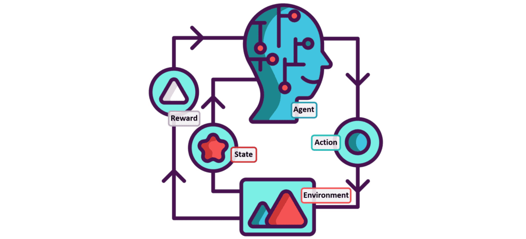
Reinforcement learning (RL) is a powerful branch of machine learning that has gained significant attention in recent years. Unlike supervised and unsupervised learning, RL focuses on learning through interaction with an environment. In this paradigm, an agent learns to make optimal decisions by receiving rewards or punishments based on its actions. The goal is to maximize the cumulative reward over time, enabling the agent to learn and adapt its behavior in complex and dynamic environments.

RL has its roots in psychology and neuroscience, drawing inspiration from how humans and animals learn through trial and error. The concept of reinforcement, where desirable behaviors are encouraged and undesirable ones are discouraged, forms the foundation of RL. By continuously exploring and exploiting its environment, an RL agent can learn to make intelligent decisions and solve complex problems.

One of the key advantages of RL is its ability to learn from sparse and delayed rewards. Unlike supervised learning, where the correct output is provided for each input, RL agents must discover the optimal actions through exploration and feedback. This allows RL to tackle problems where the optimal solution is not immediately apparent or where the consequences of actions are not immediately observable.

RL has found applications in a wide range of domains, from robotics and autonomous vehicles to game playing and recommendation systems. Its ability to learn from experience and adapt to changing environments makes it a powerful tool for solving real-world problems. In the following sections, we will dive deeper into the key concepts, algorithms, and applications of reinforcement learning.

Section 2: Markov Decision Processes

At the core of reinforcement learning lies the concept of Markov Decision Processes (MDPs). An MDP is a mathematical framework that describes the interaction between an agent and its environment. It consists of four main components: states, actions, transitions, and rewards.

States represent the different configurations or situations an agent can be in within the environment. For example, in a game of chess, each arrangement of pieces on the board represents a unique state. Actions are the choices available to the agent in each state. In the chess example, the agent’s actions would be the possible moves it can make.

Transitions define how the environment evolves from one state to another based on the agent’s actions. In an MDP, the transition probabilities satisfy the Markov property, which means that the next state depends only on the current state and the action taken, not on the history of previous states and actions.

Rewards are the feedback signals that the agent receives from the environment after taking an action. Rewards can be positive, indicating desirable outcomes, or negative, indicating undesirable ones. The goal of the agent is to maximize the cumulative reward over time.

MDPs provide a structured way to model sequential decision-making problems. By formulating a problem as an MDP, we can leverage the tools and algorithms of reinforcement learning to find optimal policies that maximize the expected cumulative reward.

One important concept in MDPs is the value function, which estimates the expected cumulative reward an agent can obtain from a given state by following a specific policy. The optimal value function corresponds to the maximum expected cumulative reward achievable from each state.

Solving an MDP involves finding the optimal policy, which maps states to actions in a way that maximizes the expected cumulative reward. Dynamic programming algorithms, such as value iteration and policy iteration, can be used to compute the optimal value function and policy for small to medium-sized MDPs.

However, in many real-world problems, the state and action spaces can be large or even continuous, making exact solutions intractable. In such cases, approximate solution methods, such as function approximation and sampling-based techniques, are employed to find good approximations of the optimal policy.

Understanding MDPs is crucial for grasping the foundations of reinforcement learning and developing effective RL algorithms. By modeling problems as MDPs and leveraging the tools and techniques of RL, we can tackle complex sequential decision-making tasks and build intelligent agents that learn from experience.

Section 3: Q-Learning

Q-learning is a popular and widely used algorithm in reinforcement learning. It is a model-free, off-policy algorithm that learns the optimal action-value function, also known as the Q-function. The Q-function represents the expected cumulative reward an agent can obtain by taking a specific action in a given state and following the optimal policy thereafter.

The key idea behind Q-learning is to iteratively update the Q-values based on the observed rewards and the maximum Q-value of the next state. The update rule for Q-learning is as follows:

Q(s, a) ← Q(s, a) + α[r + γ max_a’ Q(s’, a’) – Q(s, a)]

Here, Q(s, a) represents the current Q-value for taking action a in state s, α is the learning rate that controls the step size of the update, r is the observed reward, γ is the discount factor that balances the importance of immediate and future rewards, and max_a’ Q(s’, a’) represents the maximum Q-value for the next state s’ over all possible actions a’.

The Q-learning algorithm starts with an initialized Q-table, where each entry corresponds to a state-action pair. The agent interacts with the environment by selecting actions based on an exploration-exploitation strategy, such as ε-greedy. With probability ε, the agent explores by taking a random action, and with probability 1-ε, it exploits by choosing the action with the highest Q-value.

As the agent interacts with the environment, it updates the Q-values using the Q-learning update rule. Over time, the Q-values converge to the optimal values, and the agent learns the optimal policy by selecting the actions with the highest Q-values in each state.

Q-learning has several advantages. It is simple to implement and can handle stochastic environments with uncertain transitions and rewards. It also converges to the optimal policy under certain conditions, such as visiting each state-action pair infinitely often.

However, Q-learning can suffer from the “curse of dimensionality” when the state and action spaces are large. In such cases, function approximation techniques, such as neural networks, can be used to approximate the Q-function. This variant of Q-learning is known as Deep Q-Learning (DQN) and has achieved impressive results in complex domains like playing Atari games.

Q-learning has been successfully applied to various problems, including robot navigation, game playing, and autonomous vehicle control. Its simplicity and effectiveness make it a popular choice for many reinforcement learning tasks.

Section 4: Policy Gradients

Policy gradient methods are another class of reinforcement learning algorithms that directly optimize the policy parameters to maximize the expected cumulative reward. Unlike value-based methods like Q-learning, which learn the value function and derive the policy implicitly, policy gradient methods explicitly parameterize the policy and update its parameters based on the gradient of the expected reward.

The key idea behind policy gradient methods is to represent the policy as a differentiable function, typically a neural network, with adjustable parameters θ. The objective is to find the optimal parameters θ* that maximize the expected cumulative reward J(θ):

θ* = argmax_θ J(θ)

The gradient of the expected reward with respect to the policy parameters can be estimated using the policy gradient theorem:

∇_θ J(θ) = E_τ[∑_t ∇_θ log π_θ(a_t|s_t) Q^π(s_t, a_t)]

Here, τ represents a trajectory (a sequence of states, actions, and rewards) sampled from the policy π_θ, ∇_θ log π_θ(a_t|s_t) is the gradient of the log probability of taking action a_t in state s_t, and Q^π(s_t, a_t) is the state-action value function under the current policy.

The policy gradient theorem suggests that to maximize the expected reward, we should increase the probability of taking actions that lead to higher Q-values and decrease the probability of actions with lower Q-values. This is achieved by updating the policy parameters in the direction of the estimated gradient:

θ ← θ + α ∇_θ J(θ)

where α is the learning rate.

There are different variants of policy gradient methods, such as REINFORCE, Actor-Critic, and Proximal Policy Optimization (PPO).

Section 5: Actor-Critic Methods

Actor-Critic methods are a popular class of policy gradient algorithms that combine the advantages of both value-based and policy-based methods. They consist of two main components: an actor that learns the policy and a critic that estimates the value function.

The actor is responsible for selecting actions based on the current policy, which is typically represented by a neural network with parameters θ. The critic, on the other hand, estimates the value function (either the state-value function V(s) or the action-value function Q(s, a)) using a separate neural network with parameters w.

The critic’s role is to provide an evaluation of the actor’s policy by estimating the expected cumulative reward from each state or state-action pair. This evaluation serves as a baseline for the actor to improve its policy. The actor updates its parameters in the direction of the policy gradient, using the critic’s estimates to reduce the variance of the gradient estimates.

The update rules for the actor and critic in a basic Actor-Critic algorithm are as follows:

Actor update: θ ← θ + α_θ ∇_θ log π_θ(a_t|s_t) (R_t – V_w(s_t))
Critic update: w ← w + α_w (R_t – V_w(s_t)) ∇_w V_w(s_t)

Here, α_θ and α_w are the learning rates for the actor and critic, respectively, R_t is the cumulative reward from time step t, and V_w(s_t) is the critic’s estimate of the value function for state s_t.

The advantage of Actor-Critic methods is that they can reduce the variance of the gradient estimates by using the critic’s value estimates as a baseline. This can lead to more stable and efficient learning compared to pure policy gradient methods.

There are various extensions and improvements to the basic Actor-Critic algorithm, such as Advantage Actor-Critic (A2C), Asynchronous Advantage Actor-Critic (A3C), and Soft Actor-Critic (SAC). These algorithms incorporate techniques like parallel training, entropy regularization, and off-policy learning to further enhance the performance and stability of Actor-Critic methods.

Actor-Critic methods have been successfully applied to a wide range of reinforcement learning tasks, including continuous control problems, robotics, and game playing. They offer a powerful and flexible framework for learning policies in complex environments.

Section 6: Exploration vs Exploitation

One of the fundamental challenges in reinforcement learning is balancing exploration and exploitation. Exploration refers to the agent’s behavior of trying out new actions and visiting unfamiliar states to gather more information about the environment. Exploitation, on the other hand, involves leveraging the knowledge already acquired to make the best decisions based on the current estimates of the value function or policy.

The trade-off between exploration and exploitation is crucial because an agent that exclusively exploits its current knowledge may miss out on potentially better strategies and get stuck in suboptimal solutions. On the other hand, an agent that excessively explores may waste time and resources on unproductive actions and fail to converge to a good policy.

Various exploration strategies have been proposed to address this trade-off. One common approach is ε-greedy exploration, where the agent selects the action with the highest estimated value with probability 1-ε and takes a random action with probability ε. The value of ε can be gradually decreased over time to transition from exploration to exploitation.

Another approach is to use exploration bonuses, which add an additional reward term to encourage the agent to visit less frequently visited states or take less frequently chosen actions. This can be achieved through techniques like count-based exploration, where the agent keeps track of the visitation counts of states or state-action pairs and assigns higher bonuses to less visited ones.

More sophisticated exploration strategies, such as Upper Confidence Bound (UCB) and Thompson Sampling, leverage the uncertainty in the value estimates to guide exploration. UCB methods select actions based on an upper confidence bound of the estimated values, favoring actions with high potential rewards and high uncertainty. Thompson Sampling maintains a probability distribution over the possible optimal actions and samples actions from this distribution, naturally balancing exploration and exploitation.

In practice, the choice of exploration strategy depends on the specific problem and the available prior knowledge. It is important to find the right balance between exploration and exploitation to ensure efficient learning and convergence to a good policy.

Effective exploration is particularly challenging in large and complex environments, where the state and action spaces are vast. In such cases, more advanced exploration techniques, such as intrinsic motivation and curiosity-driven exploration, can be employed to guide the agent towards informative and promising regions of the state space.

Section 7: Deep Reinforcement Learning

Deep Reinforcement Learning (DRL) is a subfield of reinforcement learning that combines the power of deep neural networks with RL algorithms. DRL has revolutionized the field by enabling agents to learn complex policies directly from high-dimensional sensory inputs, such as images or raw sensor data.

The key idea behind DRL is to use deep neural networks as function approximators for the value function, policy, or both. Instead of maintaining tabular representations or using simple linear approximators, DRL leverages the expressive power of deep networks to learn rich and abstract representations of the environment.

One of the breakthrough algorithms in DRL is Deep Q-Networks (DQN), which extends the classical Q-learning algorithm to handle high-dimensional state spaces. DQN uses a deep neural network to approximate the Q-function, mapping states to action values. The network is trained using a variant of Q-learning, where the target Q-values are computed using a separate target network to stabilize the learning process.

Another prominent DRL algorithm is Deep Deterministic Policy Gradient (DDPG), which is an extension of the Actor-Critic method for continuous action spaces. DDPG uses two separate neural networks: an actor network that outputs continuous actions and a critic network that estimates the Q-value of state-action pairs. The actor network is updated using the policy gradient, while the critic network is trained using a modified Q-learning update.

DRL has achieved remarkable success in various domains, such as game playing, robotics, and autonomous driving. For example, DQN agents have surpassed human-level performance in playing Atari games directly from screen pixels. DDPG has been applied to complex robotic tasks, such as manipulation and locomotion, enabling robots to learn dexterous skills through trial and error.

However, DRL also faces several challenges. One challenge is the sample inefficiency of RL algorithms, as they often require a large number of interactions with the environment to learn good policies. Techniques like experience replay, where past experiences are stored and reused for training, can help mitigate this issue.

Another challenge is the instability and sensitivity of DRL algorithms to hyperparameters and network architectures. Regularization techniques, such as target networks and batch normalization, can help stabilize the learning process. Additionally, proper tuning of hyperparameters and careful design of network architectures are crucial for successful DRL applications.

Despite the challenges, DRL has opened up new possibilities for solving complex sequential decision-making problems and has become a rapidly growing area of research and application.

Section 8: Model-Based Reinforcement Learning

Model-Based Reinforcement Learning (MBRL) is a paradigm within reinforcement learning that focuses on learning a model of the environment and using it to make decisions. Unlike model-free RL, which directly learns a value function or policy from interactions with the environment, MBRL explicitly learns a model that captures the dynamics of the environment, including the state transitions and rewards.

The key idea behind MBRL is to use the learned model to simulate the environment and plan actions based on the predicted outcomes. By having an internal model of the environment, an agent can reason about the consequences of its actions and make more informed decisions without the need for extensive real-world interactions.

The process of MBRL typically involves two main components: model learning and planning. In the model learning phase, the agent interacts with the environment and collects data in the form of state-action-reward tuples. This data is used to learn a model that approximates the environment’s dynamics, often using supervised learning techniques such as regression or neural networks.

Once a model is learned, the agent can use it for planning. Planning involves using the model to simulate the environment and evaluate the expected outcomes of different action sequences. This allows the agent to look ahead and consider the long-term consequences of its actions before executing them in the real environment.

There are various approaches to planning in MBRL, such as tree search methods and trajectory optimization. Tree search methods, like Monte Carlo Tree Search (MCTS), build a search tree by simulating multiple possible action sequences and selecting the most promising ones based on the expected rewards. Trajectory optimization methods, like Model Predictive Control (MPC), optimize a sequence of actions over a finite horizon by solving an optimization problem based on the learned model.

Section 9: Real-World Applications of Reinforcement Learning

Reinforcement learning has found numerous applications in real-world domains, ranging from robotics and autonomous systems to personalized recommendations and healthcare. Let’s explore a few notable examples:

1. Robotics and Autonomous Systems:
   RL has been extensively applied in robotics to enable autonomous decision-making and control. For instance, RL algorithms have been used to train robotic arms for tasks like object manipulation, assembly, and grasping. By learning from trial and error, robots can adapt to different objects and environments, making them more versatile and efficient. RL has also been employed in autonomous vehicles to learn policies for navigation, obstacle avoidance, and traffic management.
2. Game Playing:
   RL has achieved remarkable success in game playing, particularly in complex board games like chess and Go. DeepMind’s AlphaGo, which uses deep reinforcement learning, famously defeated world champion Lee Sedol in the game of Go, showcasing the potential of RL in mastering strategic decision-making. RL has also been applied to video games, enabling agents to learn to play games directly from screen pixels and achieve superhuman performance in various Atari games.
3. Personalized Recommendations:
   RL can be used to optimize personalized recommendation systems, such as movie or product recommendations. By framing the problem as a sequential decision-making task, an RL agent can learn to recommend items that maximize user engagement and satisfaction over time. The agent can learn from user feedback and adapt its recommendations based on individual preferences and behavior patterns.
4. Healthcare:
   RL has promising applications in healthcare, particularly in areas like personalized treatment planning and drug discovery. By modeling patient trajectories as a sequential decision-making process, RL algorithms can assist in optimizing treatment strategies tailored to individual patient characteristics. RL can also be used to guide the search for new drug candidates by learning policies that maximize the expected therapeutic outcomes while minimizing adverse effects.
5. Energy Management:
   RL can be applied to optimize energy management systems, such as smart grids and renewable energy systems. By learning to make strategic decisions based on real-time energy demand, supply, and pricing data, RL agents can help balance energy production and consumption, reduce costs, and improve the efficiency of energy systems. RL can also be used to control energy storage systems, such as batteries, to maximize their utilization and prolong their lifespan.

These are just a few examples of the diverse applications of reinforcement learning in real-world scenarios. As RL continues to advance and mature, we can expect to see even more innovative and impactful applications across various domains, revolutionizing the way we solve complex decision-making problems.

Section 10: Future Directions and Challenges

Reinforcement learning has made significant strides in recent years, but there are still many exciting research directions and challenges that lie ahead. Let’s explore some of the key areas of focus for the future of RL:

1. Sample Efficiency:
   One of the major challenges in RL is the requirement for a large number of interactions with the environment to learn good policies. Improving sample efficiency is crucial for applying RL to real-world problems where data collection is costly or time-consuming. Techniques like model-based RL, off-policy learning, and transfer learning are being explored to reduce the sample complexity and enable more efficient learning.
2. Generalization and Transfer Learning:
   Another important direction is enabling RL agents to generalize their learned knowledge to new tasks and environments. Transfer learning techniques aim to leverage the knowledge gained from solving one task to accelerate learning in related tasks. This can greatly reduce the training time and make RL more practical for real-world applications where environments may change or new tasks may arise.
3. Safe and Robust RL:
   Ensuring the safety and robustness of RL agents is crucial, especially in safety-critical domains like autonomous vehicles and healthcare. Developing RL algorithms that can handle uncertainty, adapt to changing environments, and make safe decisions under various constraints is an active area of research. Techniques like constrained RL, risk-sensitive RL, and safe exploration are being explored to address these challenges.
4. Explainable and Interpretable RL:
   As RL agents become more complex and autonomous, there is a growing need for explainable and interpretable RL models. Understanding the decision-making process of RL agents is important for building trust, ensuring accountability, and facilitating human-AI collaboration. Techniques like interpretable RL, where the agent’s decision-making can be explained in human-understandable terms, are being developed to address this challenge.
5. Multi-Agent RL:
   Many real-world problems involve multiple agents interacting and making decisions in a shared environment. Multi-agent RL focuses on learning policies for agents in such settings, where agents may cooperate, compete, or coordinate with each other. Challenges in multi-agent RL include handling non-stationarity, communication, and emergent behaviors. Advances in multi-agent RL can have significant implications for applications like multi-robot systems, autonomous traffic control, and strategic decision-making.
6. Integrating RL with Other AI Techniques:
   Combining RL with other AI techniques, such as deep learning, planning, and knowledge representation, can lead to more powerful and versatile AI systems. For example, integrating RL with symbolic reasoning and knowledge bases can enable agents to make decisions based on both learned policies and explicit domain knowledge. Hybrid approaches that leverage the strengths of different AI paradigms are an exciting avenue for future research.

As the field of reinforcement learning continues to evolve, addressing these challenges and exploring new directions will be crucial for realizing the full potential of RL in solving complex real-world problems. The future of RL holds great promise for transforming various industries and shaping the way we interact with intelligent systems.

FAQs

1. Q: What is reinforcement learning and how does it differ from other machine learning paradigms?
   A: Reinforcement learning is a machine learning paradigm where an agent learns to make optimal decisions by interacting with an environment and receiving rewards or punishments based on its actions. Unlike supervised learning, which relies on labeled data, or unsupervised learning, which focuses on finding patterns in unlabeled data, reinforcement learning learns through trial and error and delayed feedback.
2. Q: What are the key components of a reinforcement learning problem?
   A: The key components of a reinforcement learning problem are the agent, the environment, states, actions, rewards, and a policy. The agent interacts with the environment by taking actions in different states, receiving rewards, and updating its policy to maximize the cumulative reward over time.
3. Q: What is the role of the value function in reinforcement learning?
   A: The value function in reinforcement learning estimates the expected cumulative reward an agent can obtain from a given state by following a specific policy. It helps the agent evaluate the goodness of states and make informed decisions. The optimal value function corresponds to the maximum expected cumulative reward achievable from each state.
4. Q: What is the exploration-exploitation trade-off in reinforcement learning?
   A: The exploration-exploitation trade-off refers to the balance between exploring new actions and states to gather information about the environment (exploration) and exploiting the current knowledge to make the best decisions based on the learned policy (exploitation). Finding the right balance is crucial for efficient learning and convergence to an optimal policy.
5. Q: What is Q-learning and how does it work?
   A: Q-learning is a popular reinforcement learning algorithm that learns the optimal action-value function (Q-function) through iterative updates. It estimates the Q-values of state-action pairs based on the observed rewards and the maximum Q-value of the next state. The agent selects actions based on an exploration-exploitation strategy and updates the Q-values using the Q-learning update rule.
6. Q: What are policy gradient methods in reinforcement learning?
   A: Policy gradient methods are a class of reinforcement learning algorithms that directly optimize the policy parameters to maximize the expected cumulative reward. They represent the policy as a differentiable function and update its parameters based on the gradient of the expected reward. Popular policy gradient methods include REINFORCE, Actor-Critic, and Proximal Policy Optimization (PPO).
7. Q: What is the role of deep learning in reinforcement learning?
   A: Deep learning has revolutionized reinforcement learning by enabling agents to learn complex policies directly from high-dimensional sensory inputs, such as images or raw sensor data. Deep reinforcement learning algorithms, such as Deep Q-Networks (DQN) and Deep Deterministic Policy Gradient (DDPG), use deep neural networks as function approximators for the value function, policy, or both.
8. Q: What are some real-world applications of reinforcement learning?
   A: Reinforcement learning has found applications in various domains, including robotics (e.g., robotic manipulation, autonomous navigation), game playing (e.g., AlphaGo, Atari games), personalized recommendations, healthcare (e.g., treatment planning, drug discovery), and energy management (e.g., smart grids, renewable energy systems).
9. Q: What are some challenges in reinforcement learning?
   A: Some challenges in reinforcement learning include sample inefficiency (requiring a large number of interactions with the environment), instability and sensitivity to hyperparameters, difficulty in generalization and transfer learning, ensuring safety and robustness, and interpretability of learned policies. Researchers are actively exploring techniques to address these challenges and improve the performance and applicability of reinforcement learning algorithms.
10. Q: What are some future directions in reinforcement learning research?
    A: Future directions in reinforcement learning research include improving sample efficiency, enabling better generalization and transfer learning, developing safe and robust RL algorithms, creating explainable and interpretable RL models, advancing multi-agent RL, and integrating RL with other AI techniques such as deep learning, planning, and knowledge representation. These research directions aim to push the boundaries of RL and unlock its potential for solving complex real-world problems.