Introduction to Q Learning

Section 1: Introduction to Q-Learning

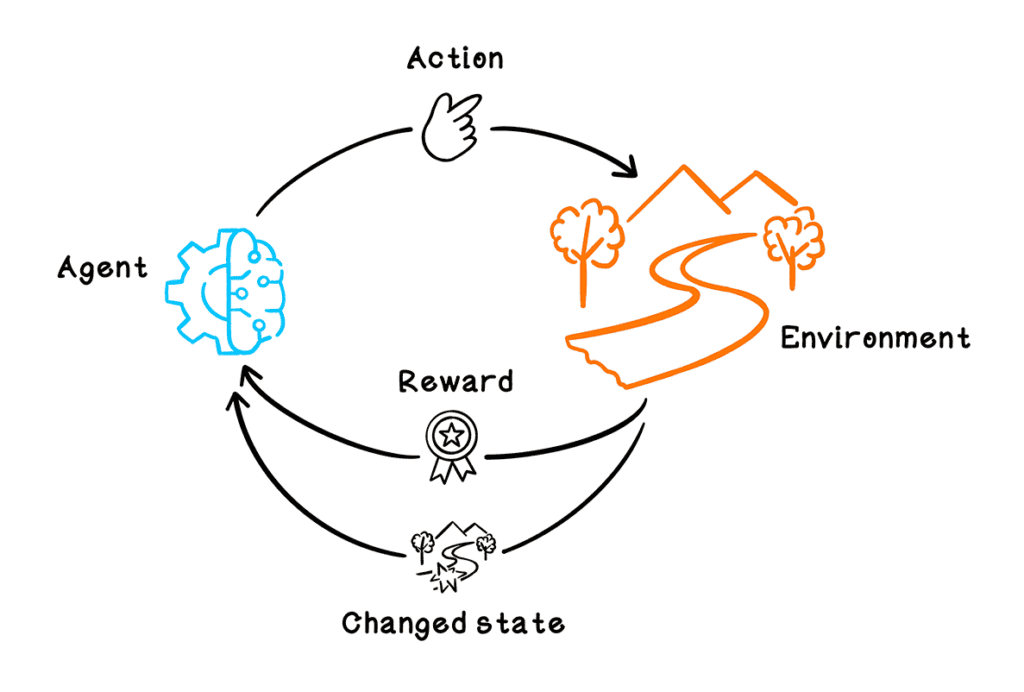
Q-Learning is a fundamental reinforcement learning algorithm in artificial intelligence that enables an agent to learn optimal decision-making through trial and error interactions with its environment. Developed by Christopher JCH Watkins in 1989, Q-Learning has become one of the most widely used and researched algorithms in the field of AI due to its simplicity, effectiveness, and wide range of applications.

At its core, Q-Learning is about learning a value function, called the Q-function, which estimates the expected cumulative reward an agent can obtain by taking a specific action in a given state and following an optimal policy thereafter. The agent’s goal is to maximize this cumulative reward over time by learning the optimal policy, i.e., the best action to take in each state.

The name “Q” in Q-Learning stands for “quality,” emphasizing the algorithm’s focus on learning the quality or value of taking an action in a particular state. By iteratively updating the Q-function based on the rewards received and the estimated future rewards, the agent gradually improves its decision-making policy and learns to navigate the environment effectively.

Q-Learning is an off-policy algorithm, meaning it can learn the optimal policy even while following a different exploration policy. This property makes Q-Learning particularly useful in situations where the optimal policy is unknown, and the agent needs to balance exploration (trying new actions) and exploitation (choosing the best action based on current knowledge).

Section 2: The Foundation of Q-Learning: Markov Decision Processes

To understand Q-Learning, it is essential first to grasp the concept of Markov Decision Processes (MDPs), which provide the mathematical framework for modeling decision-making in situations where outcomes are partly random and partly under the control of a decision-maker.

An MDP is defined by four key components:

1. States (S): A finite set of states that represent the possible configurations of the environment.
2. Actions (A): A finite set of actions the agent can take in each state.
3. Transition Probabilities (P): The probability of transitioning from one state to another when taking a specific action.
4. Rewards (R): The immediate reward received by the agent for taking an action in a given state.

The Markov property is a crucial assumption in MDPs, which states that the future state and reward depend only on the current state and action, not on the history of previous states and actions. Formally, for any state s and any action a, the probability of transitioning to state s’ and receiving reward r is given by:

P(s’,r|s,a) = P(S_{t+1}=s’, R_{t+1}=r | S_t=s, A_t=a)

This assumption simplifies the learning process, as the agent only needs to consider the current state when making decisions, rather than maintaining a complete history of past states and actions.

The goal in an MDP is to find a policy π, which is a mapping from states to actions, that maximizes the expected cumulative reward over time. The optimal policy π* is the policy that achieves the highest expected cumulative reward from any initial state.

Q-Learning is a model-free reinforcement learning algorithm that learns the optimal policy for an MDP without explicitly estimating the transition probabilities or rewards. Instead, it directly learns the Q-function, which encodes the expected cumulative reward for each state-action pair.

By understanding MDPs and their components, we lay the groundwork for exploring how Q-Learning works and how it enables an agent to learn optimal decision-making policies through interaction with its environment.

Section 3: The Q-Function and Bellman Equation

At the heart of Q-Learning lies the Q-function, which is a mapping from state-action pairs to expected cumulative rewards. The Q-function is defined as:

Q(s,a) = E[R_t + γ * max_a’ Q(s’,a’) | S_t=s, A_t=a]

where:

• s is the current state
• a is the action taken in state s
• R_t is the immediate reward received after taking action a in state s
• γ is the discount factor (between 0 and 1) that determines the importance of future rewards
• s’ is the next state after taking action a in state s
• a’ is the action taken in state s’

The Q-function represents the expected cumulative reward the agent will receive by taking action a in state s and following the optimal policy thereafter. The goal of Q-Learning is to learn this Q-function through iterative updates based on the agent’s experience.

The optimal Q-function, denoted as Q*(s,a), satisfies the Bellman equation, which is a recursive relationship that expresses the optimal Q-value of a state-action pair in terms of the optimal Q-values of the next state:

Q*(s,a) = E[R_t + γ * max_a’ Q*(s’,a’) | S_t=s, A_t=a]

The Bellman equation states that the optimal Q-value of taking action a in state s is equal to the expected immediate reward plus the discounted optimal Q-value of the next state, assuming the agent follows the optimal policy.

Q-Learning uses the Bellman equation as an iterative update rule to estimate the optimal Q-function. The Q-Learning update rule is:

Q(s,a) ← Q(s,a) + α * [R_t + γ * max_a’ Q(s’,a’) – Q(s,a)]

where α is the learning rate that controls the size of the update step.

This update rule adjusts the Q-value of the current state-action pair (s,a) towards the target value, which is the sum of the immediate reward and the discounted maximum Q-value of the next state. The learning rate α determines the extent to which the new information overrides the old Q-value estimate.

By iteratively applying this update rule, the agent gradually improves its estimate of the Q-function, eventually converging to the optimal Q-function Q*(s,a) that satisfies the Bellman equation. Once the optimal Q-function is learned, the agent can derive the optimal policy by simply selecting the action with the highest Q-value in each state:

π*(s) = argmax_a Q*(s,a)

Understanding the Q-function and the Bellman equation is crucial for grasping how Q-Learning enables an agent to learn optimal decision-making policies through experience. In the next section, we will explore the Q-Learning algorithm in detail and see how these concepts are put into practice.

Section 4: The Q-Learning Algorithm

The Q-Learning algorithm is an iterative process that allows an agent to learn the optimal Q-function and, consequently, the optimal policy for a given Markov Decision Process (MDP). The algorithm follows these steps:

1. Initialize the Q-function:
   • For all states s ∈ S and actions a ∈ A, set Q(s,a) to arbitrary initial values (e.g., 0).
2. Observe the current state s.
3. Choose an action a in state s using an exploration-exploitation strategy (e.g., ε-greedy).
4. Take action a, observe the reward r and the next state s’.
5. Update the Q-value for the state-action pair (s,a) using the Q-Learning update rule:
   Q(s,a) ← Q(s,a) + α * [r + γ * max_a’ Q(s’,a’) – Q(s,a)]
6. Set the current state s to the next state s’.
7. Repeat steps 3-6 until a termination condition is met (e.g., reaching a goal state or a maximum number of iterations).

The exploration-exploitation strategy in step 3 is crucial for balancing the agent’s need to explore the environment and discover new rewarding actions with the need to exploit its current knowledge to maximize rewards. A common strategy is ε-greedy, where the agent chooses a random action with probability ε (exploration) and the action with the highest Q-value with probability 1-ε (exploitation). The value of ε is typically decreased over time to gradually shift from exploration to exploitation.

Section 5: Exploration vs Exploitation in Q-Learning

One of the key challenges in Q-Learning is balancing exploration and exploitation. Exploration refers to the agent’s willingness to try new actions to discover potentially better strategies, while exploitation involves choosing the best action based on the current knowledge to maximize immediate rewards.

The exploration-exploitation dilemma arises because the agent must gather enough information about the environment to make informed decisions while also maximizing its cumulative reward. If the agent explores too little, it may miss out on discovering optimal strategies and get stuck in suboptimal policies. On the other hand, if the agent explores too much, it may waste time and resources on inferior actions and fail to maximize its rewards.

Several strategies have been proposed to address this dilemma, including:

1. ε-greedy: The agent chooses a random action with probability ε and the action with the highest Q-value with probability 1-ε. The value of ε is decreased over time to transition from exploration to exploitation.
2. Softmax exploration: The agent selects actions based on a probability distribution determined by the Q-values, where actions with higher Q-values have a higher probability of being chosen. The temperature parameter controls the randomness of the distribution, with higher temperatures favoring exploration and lower temperatures favoring exploitation.
3. Upper Confidence Bound (UCB): The agent selects actions based on an upper confidence bound of the Q-values, which balances the estimated Q-value with the uncertainty in the estimate. Actions with higher upper confidence bounds are preferred, encouraging exploration of less-visited state-action pairs.

The choice of exploration strategy depends on the specific problem and the desired balance between exploration and exploitation. In practice, it is common to start with a high level of exploration and gradually decrease it over time as the agent learns more about the environment.

Balancing exploration and exploitation is crucial for the agent to learn optimal policies efficiently. By carefully managing this trade-off, Q-Learning enables the agent to discover high-rewarding strategies while minimizing the time and resources spent on suboptimal actions.

Section 6: Advantages and Limitations of Q-Learning

Q-Learning has several advantages that make it a popular choice for reinforcement learning tasks:

Advantages:

1. Model-free: Q-Learning does not require a model of the environment’s transition probabilities or rewards, making it applicable to a wide range of problems where the dynamics of the environment are unknown or difficult to model.
2. Off-policy learning: Q-Learning can learn the optimal policy while following a different exploration policy, allowing the agent to gather information about the environment while still converging to the optimal policy.
3. Simplicity: The Q-Learning algorithm is relatively simple to understand and implement, making it a good starting point for learning about reinforcement learning.
4. Convergence guarantees: Under certain conditions (e.g., visiting all state-action pairs infinitely often, using a suitable learning rate), Q-Learning is guaranteed to converge to the optimal Q-function and, consequently, the optimal policy.

However, Q-Learning also has some limitations:

Limitations:

1. Curse of dimensionality: As the number of states and actions grows, the size of the Q-table (which stores the Q-values for each state-action pair) increases exponentially. This can lead to memory and computational issues, making Q-Learning impractical for large-scale problems.
2. Discrete state and action spaces: Q-Learning, in its basic form, is designed for discrete state and action spaces. Extending the algorithm to continuous domains requires additional techniques, such as function approximation or discretization of the state and action spaces.
3. Slow convergence: Q-Learning can be slow to converge, especially in environments with sparse rewards or large state-action spaces. This is because the agent needs to visit each state-action pair multiple times to accurately estimate the Q-values.
4. Overestimation bias: Q-Learning tends to overestimate the Q-values of actions due to the max operator in the update rule. This can lead to suboptimal policies and slower convergence, especially in stochastic environments.

Despite these limitations, Q-Learning remains a powerful and widely-used algorithm in reinforcement learning. Researchers have proposed various extensions and improvements to address these issues, such as Deep Q-Networks (DQN) for handling large state spaces, Double Q-Learning for reducing overestimation bias, and prioritized experience replay for more efficient learning.

By understanding the advantages and limitations of Q-Learning, researchers and practitioners can make informed decisions about when to apply the algorithm and how to adapt it to their specific problems.

Section 7: Variants and Extensions of Q-Learning

Since its introduction, Q-Learning has been the foundation for numerous variants and extensions that aim to address its limitations and improve its performance in various settings. Some notable variants and extensions include:

1. Deep Q-Networks (DQN): DQN combines Q-Learning with deep neural networks to handle large state spaces. Instead of maintaining a Q-table, DQN uses a neural network to approximate the Q-function, enabling it to learn from high-dimensional sensory inputs like images. DQN has achieved remarkable success in playing Atari games and has spawned further extensions like Double DQN and Dueling DQN.
2. Double Q-Learning: Double Q-Learning addresses the overestimation bias in Q-Learning by decoupling the action selection and value estimation steps. It maintains two separate Q-functions and uses one to select actions and the other to estimate the Q-values. This simple modification has been shown to reduce overestimation and improve the quality of learned policies.
3. Prioritized Experience Replay: In Q-Learning, the agent’s experiences (state, action, reward, next state) are typically stored in a replay buffer and sampled uniformly during training. Prioritized experience replay assigns higher sampling probabilities to experiences that are more informative (e.g., those with larger temporal-difference errors). This can accelerate learning by focusing on the most relevant experiences.
4. Multi-agent Q-Learning: Q-Learning can be extended to multi-agent settings where multiple agents interact with each other in a shared environment. Each agent learns its own Q-function while considering the actions of other agents. Extensions like Nash Q-Learning and Correlated Q-Learning have been proposed to address the challenges of multi-agent learning, such as non-stationarity and coordination.
5. Continuous action spaces: While basic Q-Learning is designed for discrete action spaces, extensions like Normalized Advantage Functions (NAF) and Deep Deterministic Policy Gradient (DDPG) enable Q-Learning to handle continuous action spaces. These methods use neural networks to parameterize the Q-function and the policy, allowing the agent to learn continuous control tasks.
6. Hierarchical Q-Learning: Hierarchical Q-Learning introduces temporal abstraction by learning a hierarchy of Q-functions operating at different time scales. The high-level Q-functions learn to select subgoals, while the low-level Q-functions learn to achieve these subgoals. This hierarchical structure can accelerate learning and enable the agent to tackle complex tasks more efficiently.

These are just a few examples of the many variants and extensions of Q-Learning that have been proposed in the literature. Each variant addresses specific challenges or extends the applicability of Q-Learning to new domains, contributing to the algorithm’s versatility and success in reinforcement learning.

Section 8: Implementing Q-Learning

To implement Q-Learning, we need to define the key components of the algorithm and translate them into code. Here’s a step-by-step guide to implementing Q-Learning in Python:

Step 1: Define the environment
First, we need to define the environment in which the agent will learn and interact. This involves specifying the state and action spaces, the transition dynamics, and the reward function. For this example, let’s consider a simple grid-world environment where the agent’s goal is to navigate from a starting state to a goal state while avoiding obstacles.

python

import numpy as np

class GridWorld:
    def __init__(self, grid):
        self.grid = grid
        self.rows, self.cols = len(grid), len(grid[0])
        self.state = None
        
    def reset(self):
        self.state = (0, 0)  # Start at the top-left corner
        return self.state
    
    def step(self, action):
        row, col = self.state
        if action == 0:  # Up
            row = max(0, row - 1)
        elif action == 1:  # Down
            row = min(self.rows - 1, row + 1)
        elif action == 2:  # Left
            col = max(0, col - 1)
        elif action == 3:  # Right
            col = min(self.cols - 1, col + 1)
        
        self.state = (row, col)
        reward = self.grid[row][col]
        done = (reward > 0)  # Terminate when reaching a positive reward
        return self.state, reward, done

Step 2: Initialize the Q-table
Next, we need to initialize the Q-table, which will store the Q-values for each state-action pair. We can represent the Q-table as a multi-dimensional array with dimensions corresponding to the state space and action space.

python

num_states = env.rows * env.cols
num_actions = 4
q_table = np.zeros((num_states, num_actions))

Step 3: Define the Q-Learning algorithm
Now, we can define the Q-Learning algorithm itself. The algorithm iteratively updates the Q-values based on the agent’s experience using the Q-Learning update rule.

python

def q_learning(env, num_episodes, alpha, gamma, epsilon):
    for episode in range(num_episodes):
        state = env.reset()
        done = False
        
        while not done:
            if np.random.uniform(0, 1) < epsilon:
                action = np.random.randint(0, num_actions)  # Explore
            else:
                action = np.argmax(q_table[state])  # Exploit
            
            next_state, reward, done = env.step(action)
            
            # Q-Learning update
            q_table[state][action] += alpha * (reward + gamma * np.max(q_table[next_state]) - q_table[state][action])
            
            state = next_state

In this implementation, we run the Q-Learning algorithm for a specified number of episodes. In each episode, the agent starts from the initial state and takes actions according to an epsilon-greedy exploration strategy. The Q-values are updated using the Q-Learning update rule, which incorporates the learning rate (alpha), discount factor (gamma), and the maximum Q-value of the next state.

Step 4: Train the agent and evaluate the learned policy
Finally, we can train the agent using the Q-Learning algorithm and evaluate the learned policy by having the agent interact with the environment.

python

# Define the grid-world environment
grid = [
    [0, 0, 0, 1],
    [0, -1, 0, 0],
    [0, 0, 0, 0],
    [0, 0, 0, 0]
]
env = GridWorld(grid)

# Set hyperparameters
num_episodes = 1000
alpha = 0.1
gamma = 0.9
epsilon = 0.1

# Train the agent
q_learning(env, num_episodes, alpha, gamma, epsilon)

# Evaluate the learned policy
state = env.reset()
done = False
while not done:
    action = np.argmax(q_table[state])
    state, reward, done = env.step(action)
    print(f"State: {state}, Action: {action}, Reward: {reward}")

In this example, we define a simple 4×4 grid-world environment with a goal state (reward = 1) and an obstacle (reward = -1). We train the agent using Q-Learning for a specified number of episodes and then evaluate the learned policy by having the agent navigate the environment using the greedy policy derived from the learned Q-values.

This implementation provides a basic framework for applying Q-Learning to a simple environment. In practice, you may need to adapt the code to handle more complex state and action spaces, incorporate function approximation for large-scale problems, and fine-tune the hyperparameters for optimal performance.

Section 9: Applications of Q-Learning

Q-Learning has been successfully applied to a wide range of problem domains, showcasing its versatility and effectiveness as a reinforcement learning algorithm. Some notable applications of Q-Learning include:

1. Game Playing: Q-Learning has been used to train agents to play various games, from simple grid-world games to complex video games. One of the most famous examples is DeepMind’s DQN agent, which learned to play Atari games at a superhuman level using Q-Learning with deep neural networks.
2. Robotics: Q-Learning has been applied to robot control tasks, enabling robots to learn optimal control policies through interaction with their environment. Examples include learning to navigate mazes, manipulate objects, and perform assembly tasks.
3. Traffic Control: Q-Learning has been used to optimize traffic signal control in urban transportation networks. By learning the optimal timing of traffic lights based on traffic flow patterns, Q-Learning can help reduce congestion and improve overall traffic efficiency.
4. Resource Management: Q-Learning has been applied to resource management problems, such as load balancing in computer clusters, energy management in smart grids, and inventory management in supply chains. By learning optimal allocation strategies, Q-Learning can help optimize resource utilization and minimize costs.
5. Recommendation Systems: Q-Learning can be used to build adaptive recommendation systems that learn user preferences through interaction. By modeling the recommendation problem as a Markov Decision Process, Q-Learning can learn to suggest items that maximize long-term user satisfaction.
6. Healthcare: Q-Learning has been explored in healthcare applications, such as optimizing treatment strategies for chronic diseases, personalizing medication dosing, and improving patient adherence to treatment plans. By learning from patient data and treatment outcomes, Q-Learning can assist in data-driven decision-making and personalized healthcare.
7. Finance: Q-Learning has been applied to financial problems, such as portfolio optimization, algorithmic trading, and risk management. By learning optimal trading strategies and adapting to market conditions, Q-Learning can help maximize returns and mitigate financial risks.

These are just a few examples of the many applications of Q-Learning. As the field of reinforcement learning continues to advance, Q-Learning and its variants are likely to find even more diverse applications across various industries and domains.

The ability of Q-Learning to learn optimal policies through interaction with the environment, without requiring explicit models of the system dynamics, makes it a powerful and flexible algorithm for solving sequential decision-making problems. As researchers and practitioners continue to push the boundaries of Q-Learning and develop new extensions and improvements, we can expect to see even more impressive applications of this fundamental reinforcement learning algorithm in the future.

Section 10: Future Directions and Research Areas

Q-Learning has been a cornerstone of reinforcement learning research since its introduction, and it continues to inspire new directions and research areas. Some of the current and future research directions related to Q-Learning include:

1. Sample Efficiency: Improving the sample efficiency of Q-Learning is an active area of research. Techniques like model-based reinforcement learning, which learns a model of the environment to generate simulated experiences, and exploration strategies that prioritize informative experiences, are being investigated to reduce the number of interactions needed for learning.
2. Transfer Learning: Transferring knowledge learned from one task to another is crucial for efficient learning in real-world scenarios. Research on transfer learning in Q-Learning aims to develop methods for leveraging previously learned Q-functions or policies to accelerate learning in new tasks with similar structures.
3. Safe and Robust Learning: Ensuring the safety and robustness of Q-Learning agents is critical for deployment in real-world applications. Research on safe exploration, risk-sensitive Q-Learning, and robust Q-Learning under model uncertainty is ongoing to develop agents that can learn safely and reliably in complex and dynamic environments.
4. Multi-Agent Q-Learning: Extending Q-Learning to multi-agent settings, where multiple agents interact and learn simultaneously, poses new challenges such as non-stationarity, coordination, and communication. Research on multi-agent Q-Learning focuses on developing algorithms that can efficiently learn in the presence of other learning agents and achieve cooperative or competitive goals.
5. Continual Learning: In real-world scenarios, agents often face a sequence of tasks or a constantly changing environment. Continual learning in Q-Learning aims to develop methods that can learn new tasks without forgetting previously learned knowledge, enabling agents to adapt and improve over time.
6. Interpretability and Explainability: As Q-Learning is applied to more complex and high-stakes domains, there is a growing need for interpretable and explainable Q-Learning models. Research on interpreting the learned Q-functions, visualizing the agent’s decision-making process, and generating human-understandable explanations is gaining attention to build trust and facilitate the deployment of Q-Learning in real-world applications.
7. These are just a few of the many exciting research directions in Q-Learning. As the field progresses, we can expect to see further advancements in sample efficiency, generalization, safety, and interpretability, pushing the boundaries of what Q-Learning can achieve and broadening its applicability to an ever-expanding range of problems.